What is Sentinel-2’s revisit time?

Sentinel-2 images a 290 km swath from a sun-synchronous orbit, and the three spacecraft between them pass over any given place every few days. This case study measures how long that wait really is, everywhere, from a pinned catalogue propagated for 14 days.

A pass counts here whenever the swath crosses a cell, by night as readily as by day, while the Multi-Spectral Instrument images only in daylight. Illumination, cloud, and the acquisition plan are all outside the scope of this example, so the maps show where a pass was possible and not where an image was taken.

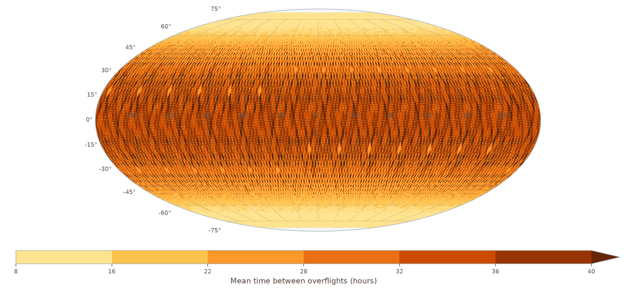
Mean time between overflights over 14 days. Consecutive one-minute intervals covered by any of the three spacecraft count as one overflight.

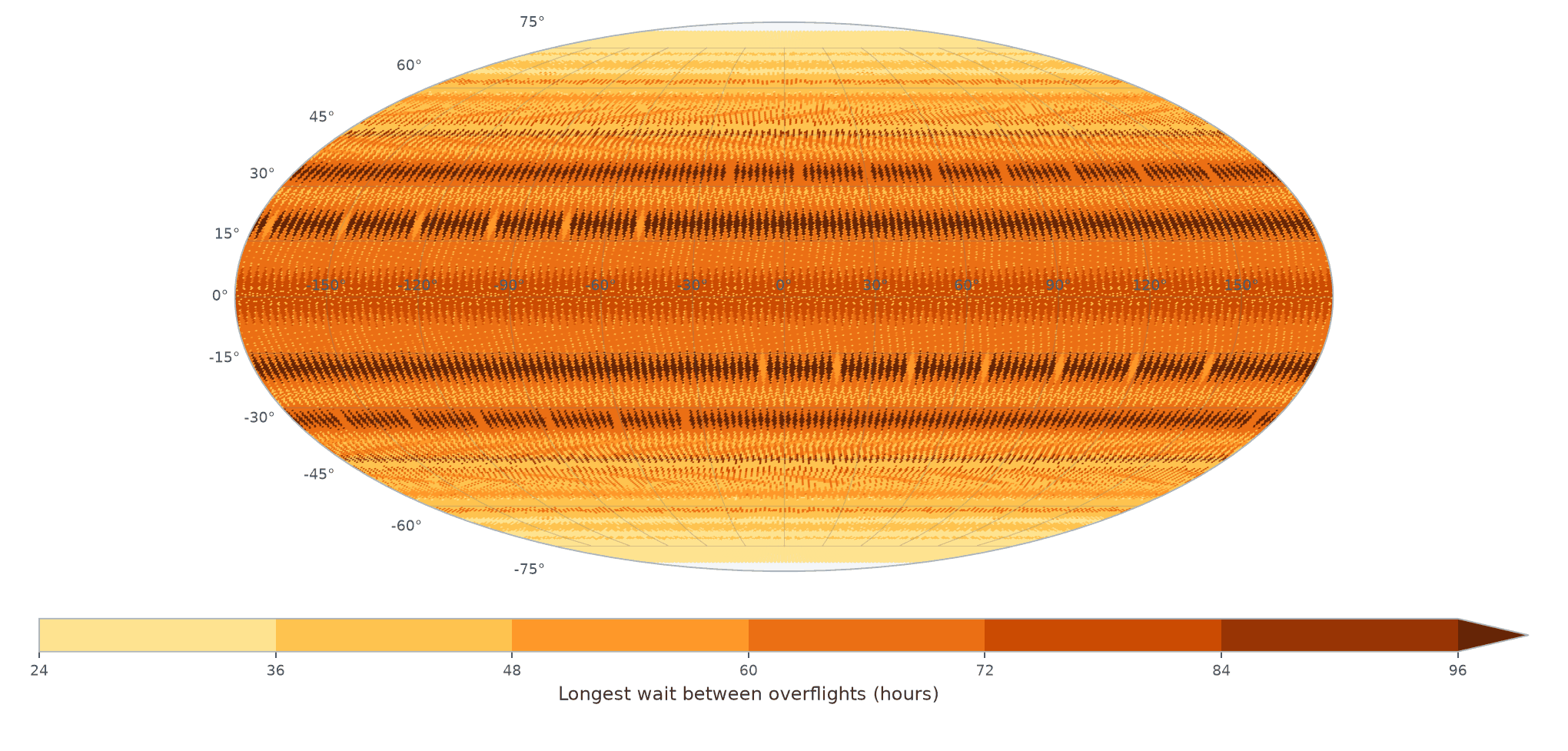
The longest single wait in the same 14 days. Waits running past the start or the end of the window are excluded, and 1,520 cells above 83° latitude are never overflown at all.

Cells near the equator wait about 37 hours between overflights, mid latitudes about 27, and the 60° to 70° band about 15, since the orbit tracks crowd together towards the poles. The longest single wait is always worse than the average: 61 hours for a typical cell, and 109 hours at the worst spot on the map.

The maps look grainy because of the grid. At 50 km cells and a 290 km swath, whether a pass catches a particular cell centre varies from one cell to the next, and a near miss moves that cell’s average by hours.

revisit() reports only complete waits between two overflights, so a cell needs at least two before it reports anything. Fourteen days is enough here: the median cell is overflown ten times, and every cell the swath reaches at all it reaches at least twice. Above 83° latitude it reaches nothing, because the orbit is inclined 98.6° and the swath is only 290 km wide.

Performance

The pinned CodSpeed run measures the EO-shaped revisit() reference workload at about 75 ms in simulation mode. That deterministic benchmark processes ten sources and 9.28 million hits; this case study uses three sources and 2.7 million hits. It is a regression reference for the same operation, not a complete-analysis wall-clock estimate.

For context, one GitHub-hosted documentation build of the complete example at the same commit produced this pipeline profile:

Stage	Time
SGP4 propagation and swath edges	10 ms
3 cover_sweep() calls	35 ms
revisit() and gap conversion	22 ms
Complete analysis	67 ms

Those wall-clock figures show the relative cost of the end-to-end stages; they are pinned to that build and are not the regression benchmark.

Method

Parameter	Value
Spacecraft	Sentinel-2A, 2B, 2C
Catalogue	CelesTrak, pinned 2026-08-24
Propagation	Astroz 0.12.0, SGP4
Analysis window	14 days from 2026-08-24 00:00 UTC
Edge cadence	60 seconds
Sweep intervals	60,480
Swath width	290 km
Grid	HEALPix resolution 7, 196,608 cells

Resolution 7 puts about 50 km between cell centres, so a 290 km swath is a few cells wide. Each one-minute interval is a quadrilateral about 400 km along track by 290 km across, and that cadence sets the precision of every wait reported here.

First we propagate the snapshot and take each spacecraft’s sub-satellite point, from which the swath edges follow:

examples/earth_observation_constellation.py

def ground_swath(
    times_min: npt.NDArray[np.float64],
) -> tuple[npt.NDArray[np.float64], npt.NDArray[np.float64]]:
    """Return the left and right swath edges of every spacecraft."""
    import astroz

    constellation = astroz.Constellation(str(TLE_PATH))
    positions_km = astroz.propagate(
        constellation,
        times_min,
        start_time=ANALYSIS_START,
        output="ecef",
    )
    sub_satellite = positions_km / np.linalg.norm(positions_km, axis=-1, keepdims=True)
    return swath_edges(sub_satellite, half_width_rad=SWATH_HALF_WIDTH_RAD)

Each spacecraft’s 20,160 intervals then go into one cover_sweep() call, which joins consecutive samples by the shorter great-circle arc:

examples/earth_observation_constellation.py

def cover_constellation(
    left_edges: npt.NDArray[np.float64],
    right_edges: npt.NDArray[np.float64],
) -> list[px.Coverage]:
    """Cover every one-minute interval of every spacecraft's swath."""
    return [
        px.cover_sweep(
            left_edges[:, satellite],
            right_edges[:, satellite],
            resolution=HEALPIX_RESOLUTION,
        )
        for satellite in range(left_edges.shape[1])
    ]

The three results share a resolution and a segment count, so revisit() reads them as aligned timelines. Consecutive covered intervals from any spacecraft count as one overflight:

examples/earth_observation_constellation.py

def overflight_gaps(
    coverages: list[px.Coverage],
) -> tuple[
    npt.NDArray[np.int64],
    npt.NDArray[np.int64],
    npt.NDArray[np.float64],
    npt.NDArray[np.float64],
]:
    """Return visited cells, their visit counts, and their gaps in hours."""
    stats = px.revisit(coverages)
    gap_counts = stats.visit_counts - 1
    measured = gap_counts > 0
    hours_per_bin = CADENCE_S / 3_600
    mean_gap_h = stats.gap_steps_total[measured] / gap_counts[measured] * hours_per_bin
    worst_gap_h = stats.gap_steps_max[measured] * hours_per_bin
    return stats.cells, stats.visit_counts, mean_gap_h, worst_gap_h

That walks the 2.7 million interval-cell hits once, keeping one accumulator per cell and never building the individual overflights. It counts in bins, not seconds, so we convert to hours ourselves.

Run the example

pixi run --environment docs docs-earth-observation
python examples/earth_observation_constellation.py \
    --mean-gap-output PATH --worst-gap-output PATH

Full source