How many Starlink satellites can you see?

Stand outside for an hour and count the Starlink satellites that climb above 25° elevation. Now do it everywhere at once: all 10,771 catalogued objects, propagated at one-minute cadence and counted cell by cell.

How many you see depends strongly on your latitude. Because the shells are inclined, the count peaks in two bands between 40° and 50° north and south, where 70 to 90 objects are in view at once. It falls to around 37 over the equator, and to about 20 near the poles.

One caveat before you read the map. An object counts when it is geometrically above the elevation mask, whether or not it is operational or has any capacity to spare. Satellite status, beams, gateways, terrain, and the atmosphere are all outside the scope of the example.

Result

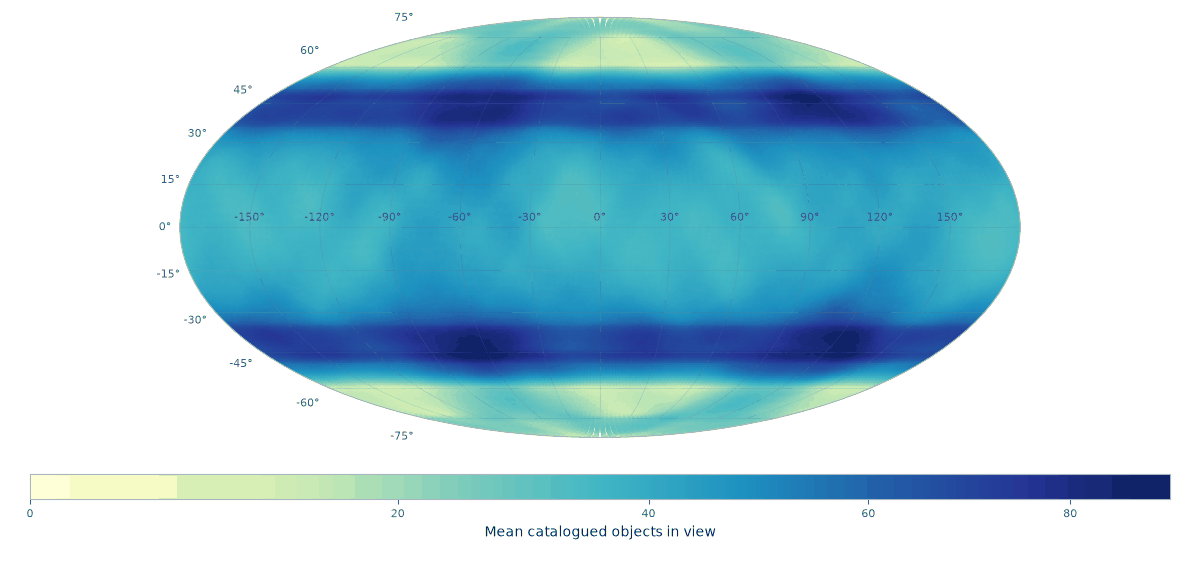
Mean simultaneous catalogued Starlink objects geometrically visible above a 25° elevation mask, sampled once per minute for one hour.

Performance

The pinned CodSpeed run measures one single-threaded timestamp of this workload—10,771 caps at resolution 6 with dense Count() reduction—at about 32 ms in simulation mode. The case study repeats that public call for 61 timestamps. This is a stable regression reference, not wall-clock time promised for a particular machine; propagation and plotting are outside the benchmark definition.

For context, one GitHub-hosted documentation build of the complete example at the same commit produced this pipeline profile:

Stage	Time
Parse pinned TLE snapshot	23 ms
SGP4 propagation	9 ms
61 cap builds and cover_cap(reduce=Count()) calls	261 ms
Complete analysis	296 ms

Those wall-clock figures show where the end-to-end work goes; they are pinned to that build for reproducibility and are not the regression benchmark.

Method

Parameter	Value
Catalog	10,771 objects, pinned 2026-07-29
Propagation	Astroz 0.12.0, SGP4
Analysis window	1 hour from 2026-07-29 00:00 UTC
Cadence	60 seconds, 61 samples
Minimum elevation	25°
Grid	HEALPix resolution 6, 49,152 cells

Resolution 6 puts roughly 100 km between cell centres, which is fine enough here. A satellite 550 km up with a 25° mask serves a circle about 1,900 km across, so one cap lands on a couple of hundred cells; across this run the average was 209. Remember that a cell is counted when its own centre falls inside a cap, which makes the map a grid of sample points and not an area intersection. Center-sampled coverage has the details, and Picking one covers the choice of resolution.

The TLE snapshot is committed to the repository. Pinning both the catalogue and the analysis time keeps the example reproducible, and keeps the documentation build off the network.

Astroz parses the snapshot and propagates every object to every timestamp, giving Earth-fixed positions in kilometres. Each of those positions then has to become a region. A satellite is visible from everywhere inside a circle on the ground, and how wide that circle is depends on how high the satellite is, so the radius comes out of the orbit radius and the elevation mask:

examples/constellation.py

def service_caps(
    positions_km: npt.NDArray[np.float64],
    *,
    body_radius_km: float,
    minimum_elevation_rad: float,
) -> tuple[npt.NDArray[np.float64], npt.NDArray[np.float64]]:
    """Return ground-service cap centers and altitude-dependent radii."""
    orbit_radii_km = np.linalg.norm(positions_km, axis=1)
    centers = positions_km / orbit_radii_km[:, np.newaxis]
    radii = (
        np.arccos(
            np.clip(
                body_radius_km / orbit_radii_km * math.cos(minimum_elevation_rad),
                -1.0,
                1.0,
            )
        )
        - minimum_elevation_rad
    )
    return centers, radii

That is the whole conversion from a propagated state to something Polypix accepts: an array of centre directions and an array of radii in radians. All 10,771 of them at one timestamp then go into a single call:

examples/communication_constellation.py

def count_visible(
    snapshot_positions_km: npt.NDArray[np.float64],
    *,
    resolution: int = HEALPIX_RESOLUTION,
    candidate_cells: npt.NDArray[np.int64] | None = None,
) -> npt.NDArray[np.int64]:
    """Count the objects in view of every cell, at one timestamp."""
    centers, radii_rad = service_caps(
        snapshot_positions_km,
        body_radius_km=EARTH_RADIUS_KM,
        minimum_elevation_rad=MINIMUM_ELEVATION_RAD,
    )
    return px.cover_cap(
        centers,
        radii_rad,
        resolution=resolution,
        candidate_cells=candidate_cells,
        reduce=px.Count(),
    )

reduce=px.Count() is what makes this cheap. Asking for counts instead of membership lets the cap kernel consume analytic RING spans, so it never builds the cap-cell pairs at all. Over the hour that is 657,031 caps and 137 million cap-cell hits, none of which is ever stored: the running total is one array of 49,152 integers.

Analyze only Germany

Now, we take the same Starlink example, butj only want analyze the results for Germany.

examples/communication_constellation.py

def germany_cells() -> npt.NDArray[np.int64]:
    """Return the resolution-9 cells whose centres lie inside Germany."""
    longitude, latitude = np.radians(GERMANY_BOUNDARY_LON_LAT_DEG).T
    boundary = np.column_stack(
        (
            np.cos(latitude) * np.cos(longitude),
            np.cos(latitude) * np.sin(longitude),
            np.sin(latitude),
        )
    )
    return px.cover_polygon(px.Polygon(boundary), resolution=GERMANY_RESOLUTION).cells

Then pass those cells through the same analysis:

aoi_cells = germany_cells()
germany = analyze(resolution=GERMANY_RESOLUTION, candidate_cells=aoi_cells)

germany.mean_visible now has one value per cell in aoi_cells, in the same order.

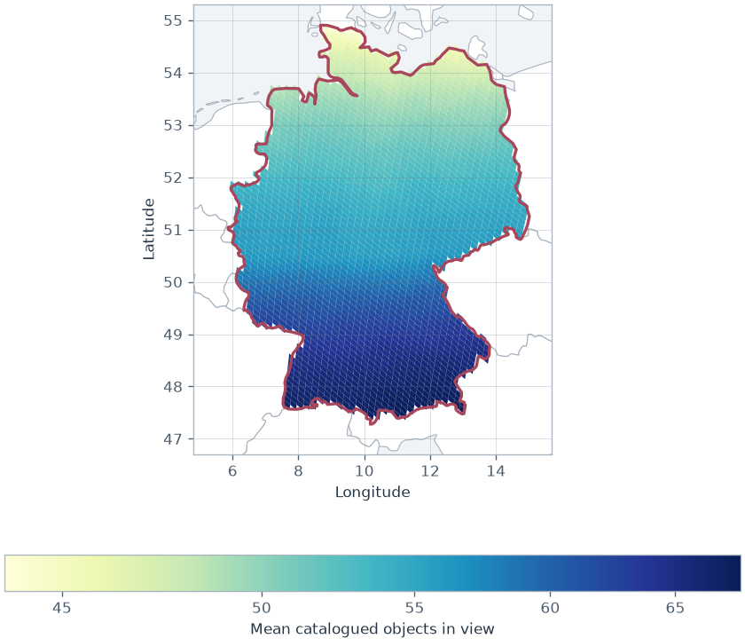
Mean simultaneous catalogued Starlink objects visible above 25° within the Germany area of interest. The red line shows the concave polygon supplied to cover_polygon().

This uses resolution 9, with roughly 13 km between neighboring cell centers. The boundary is a bundled Natural Earth extract, so the example remains reproducible and does not download map data while building the docs.

The selected-cell path is covered by the same public CodSpeed suite. Its exact cost depends on how many cells are requested, so this example makes no separate wall-clock claim for Germany.

Run the example

pixi run --environment docs docs-communications
python examples/communication_constellation.py --output PATH

Full example source

Adapting it

The scenario is four constants and a catalogue, so the interesting variations are cheap:

• Change MINIMUM_ELEVATION_RAD for a different mask. The cap radius follows from it, and no other part of the example needs to know.

• Swap the TLE file for your own catalogue, or propagate with whatever you already use. Polypix only ever sees centres and radii.

• Restrict the answer to a service area by passing candidate_cells= to cover_cap(), which is what you want when the grid is large and the region of interest is not.

• Raise HEALPIX_RESOLUTION for finer cells, remembering that each step up quadruples the count.